When you first dive into State Estimation and Kalman Filters (whether Extended or Unscented), you learn that they belong to a broader family of Gaussian Filters. But soon enough, a close cousin is introduced: the Information Filter.
This alternative view makes you realize that a Gaussian distribution actually has two equally valid, dual descriptions:
- The Moment Form: The one we are most familiar with, parameterized by a mean and a covariance (μ, Σ).
- The Information Form: The canonical view, parameterized by an information vector and an information matrix (η, Λ).
The Duality: Bells vs. Bowls
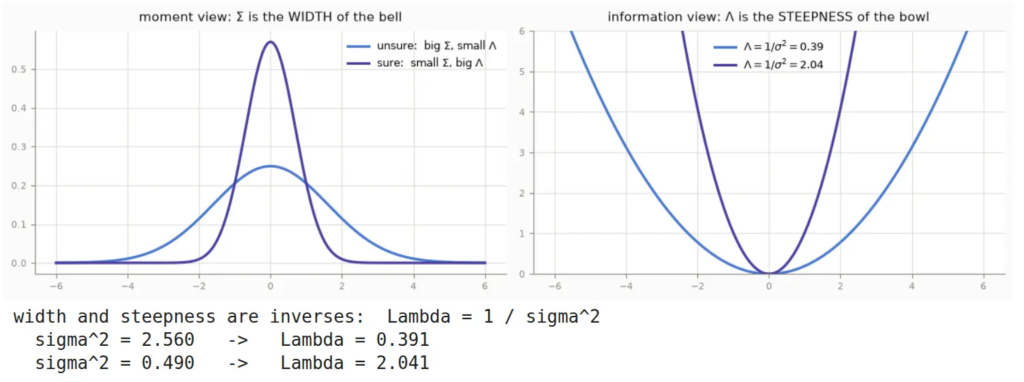
The beautiful thing about these two forms is that they are mirror images of each other. Think of it physically: the covariance Σ represents the width of the bell curve. A wide, flat bell curve means high uncertainty.
Conversely, the information matrix Λ (also known as the precision matrix) is the inverse of the covariance (Λ = Σ^-1). It represents the steepness of the bowl resulting from the negative log-likelihood -log p(x).

When your uncertainty shrinks (creating a tall, certain bell curve), your information matrix increases, meaning the negative-log cost rises sharply because you are highly certain about the state (view Figure 1).
The Algorithmic Trade-Off
For classic filtering, this duality creates an interesting computational trade-off:
- The Prediction Step: In the classic Kalman Filter, predicting the next state is largely additive and computationally cheap. In the Information Filter, prediction is a nightmare because it requires inverting matrices to pass the uncertainty forward.
- The Update Step (Sensor Fusion): This is where the tables turn. The Kalman Filter requires a costly matrix inversion to compute the Kalman Gain. The Information Filter, however, handles updates via pure addition (Λ_fused = Λ_1 + Λ_2). You simply sum the running certainties and the running directional pulls.
Connecting the Dots to Factor Graphs
This exact additivity is why the entire world of modern SLAM and Factor Graphs lives inside the information form: fusion is simply addition.
The true superpower of Factor Graphs lies in their ability to elegantly fuse asynchronous data from disparate sensors — including sensors that might drop offline for extended periods (like a GPS outage) and magically reappear. To do this efficiently, Factor Graphs exploit the anatomy of the information matrix:
- Sparsity is the Graph: Unlike the covariance matrix Σ, which becomes completely dense because everything eventually correlates over time, the information matrix Λ stays beautifully sparse. A zero entry (Λ_ij = 0) explicitly means that variable i and variable j are conditionally independent. If two states never shared a sensor measurement or a motion factor, they don’t talk to each other directly, and their corresponding block in the matrix remains zero.
- Cheap Matrix Anatomy: The two fundamental operations you ever ask of a joint Gaussian — marginalizing a variable out (forgetting it) or conditioning on a variable (pinning it down with a known measurement) — are each trivial in exactly one of the two forms. While conditioning is a free “read-off” of a block in the information form, marginalization requires a Schur complement, which structurally alters the matrix by creating “fill-in” edges between the remaining variables.
By treating the information matrix as a literal graph, we can seamlessly add new factors, remove old ones, or optimize the entire history of a robot’s trajectory using simple, sparse linear algebra.
Check out the full breakdown (with code) in the notebook below!
Leave a Reply