Making Your State Estimator ROS 2 Compliant (REP-105)

I have been having so much fun building and testing my custom state estimator. Although I am designing it to be framework-agnostic, I am building a dedicated ROS 2 layer. ROS 2 is the obvious choice for prototyping the System 1 / System 2 (Physical AI, Embodied AI, or whatever trendy term you prefer) architecture.

Clearly, the state estimator acts as a core component of a robot’s navigation stack. I am not entirely convinced that Nav2—the standard navigation stack for ROS 2—is the definitive choice for System 1 / System 2 research, given that it is built around the classical “sense-think-act” robotics loop. Nevertheless, I need to validate my estimator against it to determine whether Nav2 is a keeper or something we will need to replace moving forward.

To make any state estimation algorithm compatible with Nav2 and the broader ROS 2 ecosystem, it must comply with REP-105.

REP stands for ROS Enhancement Proposal. These are design and standard documents used to establish coding conventions, propose new features, or define technical specifications for the ROS community. REP-105 specifically defines the naming conventions and semantic meanings for the coordinate frames of mobile platforms. While it explicitly mentions mobile robots, almost every other robotic embodiment uses REP-105 with very minor modifications.

The Coordinate Frame Chain

The core philosophy of REP-105 is that there is a strict chain of navigation frames you must respect:

This setup is required for two reasons:

1. The Single Parent Rule: In ROS 2, the transform tree structure dictates that a coordinate frame can only ever have one parent.
2. Trajectory Smoothness: Navigation algorithms (like planners and controllers) require a smooth, continuous stream of positional data to avoid producing dangerous, unexpected physical movements.

Let’s define what these frames actually mean:

• base_link (or base_footprint): This frame is rigidly attached to the robot chassis. base_link usually sits at the physical center of rotation, while base_footprint is its 2D projection directly on the ground plane below the robot.
• odom: A short-term, locally consistent frame calculated via high-frequency dead reckoning. It is guaranteed to be continuous (no sudden jumps), but it will naturally drift over time due to physical factors like wheel slip.
• map: A long-term, globally consistent frame fixed to the environment. It provides an absolute coordinate system that does not drift, though transforms within it may experience sudden “jumps” when global corrections occur.
• earth: The global anchor system (such as UTM or ECEF) used to bind the local robot map to real-world geographical coordinates on the planet.

Why a Two-Stage Estimator Wins

To be ROS 2 compatible, your state estimator needs to publish these frames and respect the hierarchy. But more importantly, you can think of a good estimator as operating in two distinct stages (often running as two separate nodes).

Stage 1: The Local Estimator

The local estimator is a dead-reckoning engine. It consumes high-frequency wheel odometry and IMU data to produce a continuous, ultra-smooth estimate of the robot’s pose. This plays beautifully with local path planners and controllers. This stage publishes the odom -> base_link transform, informing the navigation stack of how the robot is moving relative to where it started.

However, as we know, without a global anchor, this odometry inevitably drifts over time due to wheel slippage and other physical phenomena.

Stage 2: The Global Estimator

This stage fuses your smooth dead-reckoning data with lower-frequency global updates from sensors like GPS or LiDAR. Because of the nature of these sensors—GPS fixes jump around due to satellite availability, and LiDAR matching can have frame-to-frame alignment errors—this global pose estimate is not smooth. It contains sudden jumps and zig-zags.

Local planners and controllers handle these jumps poorly; because they rely on smooth derivatives to calculate velocity, a sudden positional jump registers as an infinite velocity spike, causing the robot to jerk violently or trigger a safety fault.

In my original implementation, I handled this by pre-smoothing the GPS data and opting for a differential version of LiDAR odometry rather than an absolute one. REP-105 handles this in a much more elegant, albeit slightly abstract way.

By forcing a chain of transforms, my estimator behaves like two separate nodes (similar to the popular robot_localization package):

• The Local Estimator handles the fast, smooth odom -> base_link transform.
• The Global Estimator calculates where the robot actually is in the world, and publishes a map -> odom transform. This transform essentially acts as an elastic band, adjusting dynamically to cancel out wheel drift by shifting the entire local world framework.

With this separation, Nav2 stays perfectly happy. The local planners handle smooth trajectory tracking via odom -> base_link, while the map -> odom transform keeps physical reality in check by sliding the robot back into its true global position.

What about the earth frame?

The earth frame comes into play when GPS is available. The very first valid GPS fix we obtain (the datum) becomes the origin of our local map frame relative to the globe. Because GPS is noisy, we fuse it downstream, meaning there will be a small, static offset between the exact global coordinates and our map origin.

For a single robot navigating a local environment, the earth frame isn’t incredibly vital. Its true power shines in multi-robot setups where multiple vehicles need a shared global coordinate system to collaborate across massive geographical distances.

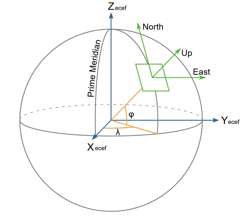
Validating the System in Simulation

With the code rewritten to comply with REP-105, the next obvious step was validation. Fortunately, I am working with the digital twin of my R1 robot rather than the massive physical hardware, allowing me to safely run three critical tests:

1. The Structural Audit (view_frames)

I ran the ROS introspection tool via the terminal:

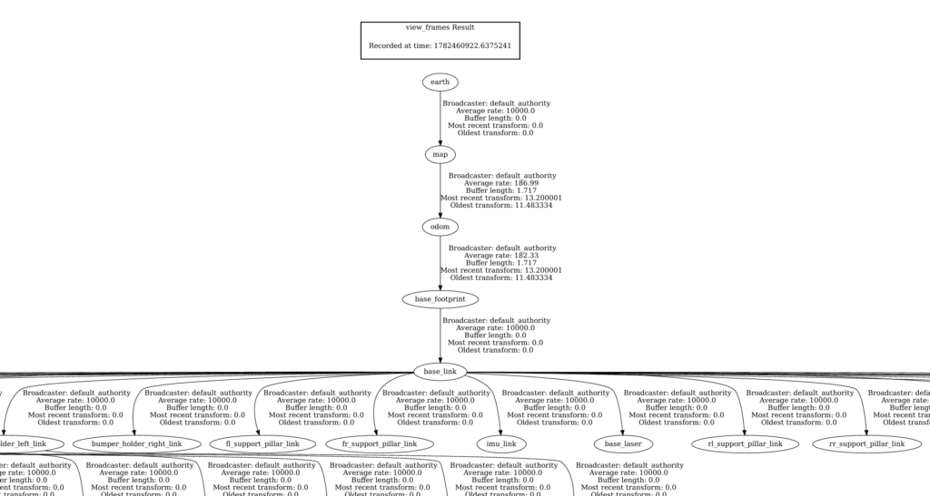
ros2 run tf2_tools view_frames

This generates a PDF mapping out the active tree. A portion of this PDF is shown in the image below. We can verify that there are no broken links, no duplicate parents, and that the hierarchy perfectly mirrors the REP-105 specification. This test passed cleanly.

2. The “Wheel Slip” Test

This test ensures that the global correction applied between map and odom is working correctly in real time. I used a classic simulation trick (that I have shown in past articles): flooring the robot directly into a sidewalk to cause extreme wheel slip.

You can see this verification in the video below. With RViz’s fixed frame set to map, the wheels keep spinning, and the local odometry believed the robot was driving forward. However, because the global estimator accurately saw the robot was physically stuck, the subtraction math kicked in. You can visually observe the odom frame marching backward through the environment while the robot (base_footprint) remained perfectly stationary on the map. The global layer successfully isolated the wheel error.

3. The “Kidnapped Robot” Test

This test ensures that a massive, sudden global position correction won’t break our local control loops. To perform this test, I used the simulation environment to “teleport” the robot several meters away.

As you can see in the video below, the result was exactly what the math ordered: the odom frame moved perfectly alongside the base_footprint frame, ensuring zero local jump during the teleportation. Meanwhile, the map -> odom transform instantly absorbed the multi-meter gap. From the perspective of the local path planner, nothing jarring occurred, allowing the robot to continue steering smoothly without crashing the navigation stack.

Architectural Peace of Mind

By letting the map -> odom transform absorb the chaos of the physical world, we achieve the ultimate balance in mobile robotics: a control loop that experiences a perfectly smooth, continuous reality, and a localization system that remains fundamentally anchored to the truth.

But Wait… How Does the Robot Actually Navigate?

Now, an interesting question arises: if all local planning and navigation steering commands are happening with respect to a drifting, technically “erroneous” odometry frame (the odom -> base_link transform), how does this affect the actual global localization? Does the robot get lost?

Amazingly, no! And this is the true mathematical beauty of the REP 105 transform tree structure.

When Nav2 plans a global path across your map, that path is generated entirely in coordinates relative to the static map frame. However, when Nav2 passes those upcoming waypoints down to the local controller to generate wheel speeds, the controller automatically transforms those global coordinates into the local odom frame using the full chain.

Because the accumulated drift error inside the odom -> base_link transform is mathematically identical to the corrective offset calculated inside the map -> odom transform, the two values perfectly cancel each other out during matrix multiplication. The local path controller might be doing its math inside a coordinate system that is sliding through space, but because the target path waypoints are being shifted by that exact same sliding vector, the physical robot still drives precisely where it needs to go in the real world. By letting the map -> odom transform absorb the chaos of sensor corrections, we achieve the ultimate robotic balance: local control loops get a smooth, continuous trajectory, while the global system stays securely anchored to physical reality.