In a previous breakdown, we explored how the classic Extended Kalman Filter (EKF) can be viewed as an optimized, local version of a factor graph, where an EKF update is essentially a single, two-factor graph solve.
As we push deeper into Factor Graphs for State Estimation, SLAM, and auto-calibration, a powerful paradigm shift emerges:
A Batch Smoother / SLAM Solve = Repeated Gauss–Newton on a Stack of Factors
By transitioning from a single execution to an iterative loop, we build a batch smoother. While the EKF linearizes exactly once at the prior mean and permanently bakes that approximation into the state estimate, an iterative Gauss-Newton engine relinearizes at each new estimate. This lets the optimizer actively “chase” the moving linearization, preventing highly nonlinear systems from accumulating errors and catastrophically diverging.
However, because this inner loop relies on a local first-order Taylor model to calculate its next step, a raw Gauss-Newton solver faces two fatal real-world vulnerabilities:
- Catastrophic Overshooting: Far from the solution, the linear model overpromises and can cause the state to blow up.
- Outlier Vulnerability: A single bad sensor reading can completely hijack the quadratic cost function.
Here is how modern estimation engines immunize themselves against both.
1. Levenberg–Marquardt: Damping the Step
A raw Gauss-Newton step trusts its local linear approximation completely. When your initial guess is far from the true solution, this approximation fails spectacularly, leading to massive overshoots or numerical failures like a LinAlgError during matrix inversion.
The Levenberg–Marquardt (LM) algorithm introduces a safety net by adding a damping term (λ) to the normal equations:
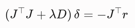
This damping factor acts as an algorithmic trust-region control:
- λ → 0: The system reverts to a standard Gauss-Newton step, fully trusting the quadratic model for rapid, superlinear convergence near the minimum.
- λ → ∞: The step scales down and aligns with the steepest gradient descent direction.
By dynamically adjusting λ based on whether a step successfully reduces the cost, the LM loop guarantees a monotonic descent downhill, elegantly handling hostile initial guesses that would send a raw Gauss-Newton solver flying off a cliff.
2. Robust Kernels: Defeating the Outliers
Standard least-squares optimization penalizes errors quadratically. If a typical clean measurement has a residual of 1σ, it contributes 1 to the cost. If a GPS multipath reflection or a bad visual loop-closure creates a 100σ blunder, it contributes 10,000 to the cost. That single corrupted measurement will completely dominate the optimization, pulling the entire trajectory off course.
To fix this, we replace the squared cost with an M-estimator, such as the Huber Kernel. The Huber kernel preserves standard quadratic least-squares for small residuals within a trusted band (|e| ≤ δ), but switches to a safer linear penalty for errors outside that band (|e| ≥ δ). This effectively caps the maximum “influence” (or pull) an outlier can exert on the system.
The Implementation Secret: “Square-Rooting the Kernel”
The most elegant part of this architecture is how it is seamlessly integrated into a standard least-squares solver using Iteratively Reweighted Least Squares (IRLS).
Mathematically, a robust M-estimator can be framed as a weighted least-squares problem where a penalty weight (w_i) is applied to the squared residual (w_i • r_i²).
However, standard linear least-squares solvers square the inputs themselves. Therefore, we cannot just pass the raw weight to the solver. Instead, we must multiply both the residual row r_i and its corresponding Jacobian row J_i by the square root of that weight.
This gives us our scaled system:

When the linear solver squares the modified residual, the square root cancels out perfectly:

This simple trick allows an ordinary, unmodified linear regression engine to minimize a robust cost function behind the scenes with zero architectural changes.
Link to the full interactive notebook with the math and Python code:
Leave a Reply