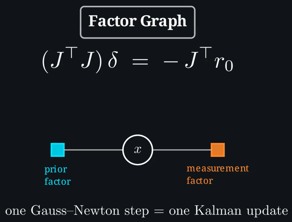
The classical Kalman Filter was an engineering shortcut designed for an era when compute was severely limited and maintaining a history of past sensor measurements was too costly. It leveraged Bayes’ rule and the Markov property to exploit the fact that the present state only depends on the immediate past, condensing the robot’s entire history into a single mean and covariance. While efficient, this recursive blending means you only get one chance to linearize your data, which permanently bakes linearization errors into your system.
Modern compute makes it entirely viable to drop these constraints, allowing us to maintain a sliding window of historical states and exploit the full power of Factor Graphs. By reframing estimation as a nonlinear least-squares optimization problem, we can continuously re-linearize past states as new information arrives. This is a significant advantage for highly nonlinear sensor models, extrinsic auto-calibration, SLAM, and handling asynchronous, slower streams of data.
The notebook below shows the exact mathematical proof, complete with live Python code, verifying that a single Extended Kalman Filter update is identical to one Gauss-Newton step on a tiny least-squares problem with just two factors: a prior factor and a measurement factor.
Leave a Reply